Examples¶

We’ll watch coastline movement from longshore drift on Cape Cod, Massachusetts, USA.

We’ll make quarterly, cloud-free-ish composites of Sentinel-2 imagery from AWS. Then turn them into GIFs.

[1]:

import pystac_client
import stackstac
import dask.array as da
import distributed
from geogif import gif, dgif

Launch a local Dask cluster. (This would be much faster with a cluster in the cloud, FWIW.)

[2]:

client = distributed.Client()

Search for STAC items overlapping our area of interest, from AWS’s open data catalog.

[3]:

bbox = (-70.05487089045347, 41.59659777453696, -69.8481905926019, 41.69921590764708)

[4]:

%%time
items = (
    pystac_client.Client.open("https://earth-search.aws.element84.com/v1")
    .search(
        bbox=bbox,
        collections=["sentinel-2-l2a"],
        datetime="2018-01-01/2024-01-01",
    )
).item_collection()

CPU times: user 1.41 s, sys: 167 ms, total: 1.57 s
Wall time: 5.9 s

Make quarterly median composites¶

Turn STAC items into xarray as a temporal stack, using stackstac.

Then mask out bad (cloudy) pixels, according to the Sentinel-2 SCL Scene Classification Map, and take the temporal median of each quarter (three months) to hopefully get an okay-looking cloud-free frame representative of those three months.

Each 3-month composite will be one frame in our animation. We end up with 18 frames.

[5]:

stack = stackstac.stack(items, bounds_latlon=bbox, resolution=30)

scl = stack.sel(band=["scl"])
# Sentinel-2 Scene Classification Map: nodata, saturated/defective, dark, cloud shadow, cloud med. prob., cloud high prob., cirrus
invalid = da.isin(scl, [0, 1, 2, 3, 8, 9, 10])
valid = stack.where(~invalid)

rgb = valid.sel(band=["red", "green", "blue"])

quarterly = rgb.resample(time="Q").median()
quarterly

[5]:

<xarray.DataArray 'stackstac-706a4f359b3be98237baef766ab69231' (time: 24,
                                                                band: 3,
                                                                y: 387, x: 579)>
dask.array<stack, shape=(24, 3, 387, 579), dtype=float64, chunksize=(1, 1, 387, 579), chunktype=numpy.ndarray>
Coordinates: (12/21)
  * time                                     (time) datetime64[ns] 2018-03-31...
  * band                                     (band) <U12 'red' 'green' 'blue'
  * x                                        (x) float64 4.121e+05 ... 4.294e+05
  * y                                        (y) float64 4.617e+06 ... 4.605e+06
    mgrs:utm_zone                            int64 19
    proj:epsg                                int64 32619
    ...                                       ...
    raster:bands                             (band) object None None None
    gsd                                      (band) object 10 10 10
    common_name                              (band) object 'red' 'green' 'blue'
    center_wavelength                        (band) object 0.665 0.56 0.49
    full_width_half_max                      (band) object 0.038 0.045 0.098
    epsg                                     int64 32619

Use .persist() to start the computation (which takes ~5min on my home internet connection, downloading ~2.5gb of data), then hold the pre-computed composites in the cluster’s memory. We’re going to reuse the same composites a few times, so it makes sense to persist it.

[6]:

ts = quarterly.persist()

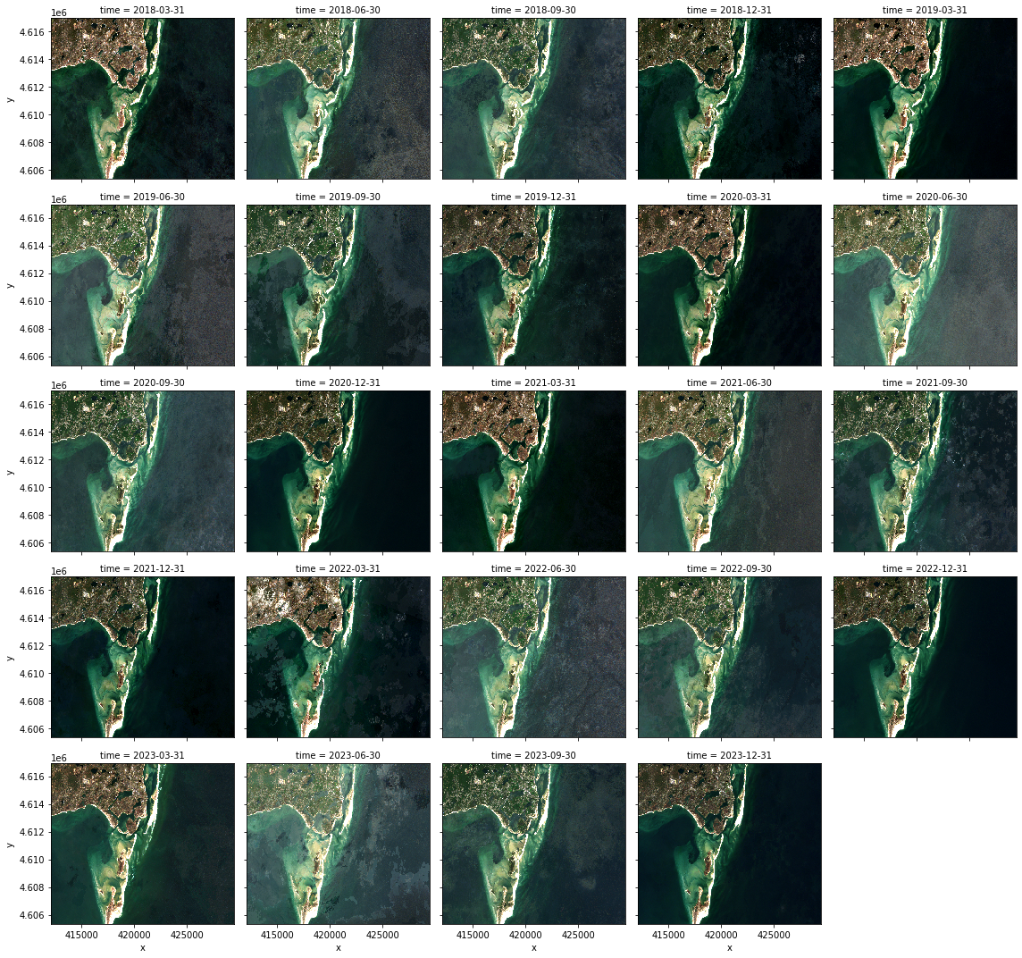
Quick filmstrip of all the frames, to see what we’re dealing with¶

We’re just showing it here for comparison to the animations.

This is actually slower than computing a GIF itself, especially if you use a remote cluster, since you have to download the full-bit-depth data from the cluster. On a cluster running in the cloud close to the imagery data, transferring this full array data can take longer than the computation itself, depending on your internet speeds.

[7]:

ts_local = ts.compute()

[8]:

ts_local.plot.imshow(col="time", rgb="band", col_wrap=5, robust=True)

[8]:

<xarray.plot.facetgrid.FacetGrid at 0x133fc2c70>

Clean up NaNs¶

Forward-fill, the backwards-fill the NaNs, to make a smoother-looking animation. (Note that this requires Bottleneck.)

[9]:

cleaned = ts.ffill("time").bfill("time")

Make GIFs!¶

Defaults¶

[10]:

dgif(cleaned).compute()

[10]:

No timestamp¶

[11]:

dgif(cleaned, date_format=None).compute()

[11]:

Big timestamp¶

[12]:

dgif(cleaned, date_size=0.5).compute()

[12]:

S L O W M O T I O N¶

[13]:

dgif(cleaned, fps=5).compute()

[13]:

`gif` (non-Dask)¶

gif and dgif behave the same. dgif(x).compute() is usually faster than gif(x.compute()).

[14]:

gif(ts_local)

[14]:

`gif` to file¶

[15]:

gif(ts_local, to="capecod.gif")

`dgif` to bytes¶

[16]:

gif_bytes = dgif(cleaned, bytes=True).compute()

[17]:

with open("capecod2.gif", "wb") as f:
    f.write(gif_bytes)

Colormapped (single-band) GIF¶

We’ll demonstrate single-band colormapped GIFs by just looking at the green band.

(Typically, you’d do something more meaningful like a derived index, but green happens to look cool in this example.)

[18]:

green = ts_local.sel(band='green')

The colormap defaults to viridis

[19]:

gif(green)

[19]:

Pick a colormap¶

[20]:

gif(green, cmap="Greens")

[20]:

Custom date format and position¶

[21]:

gif(green, date_format="Green: %Y", date_position="lr")

[21]:

Custom date color and background¶

[22]:

gif(green, date_color=(0, 10, 0), date_bg=(230, 255, 230), date_position="lr")

[22]:

Custom date color, no background, absolute font size¶

[23]:

gif(green, date_color=(0, 200, 0), date_bg=None, date_size=32, date_position="lr")

[23]: